
PID control — proportional, integral, derivative — is the workhorse of industrial process control. Most of the loops in a typical plant, from temperature and pressure to flow and level, are regulated by some form of PID controller running inside a PLC, DCS, or standalone controller. Tuning a PID loop means choosing three coefficients (Kp, Ti, Td, or their vendor-specific equivalents) so that the loop responds quickly, settles without excessive oscillation, and rejects disturbances. This article explains the terms, the standard tuning methods, and the practical steps to tune a loop on a live plant.
Understanding the Three Terms
| Term | Effect | Too much | Too little |
|---|---|---|---|
| Proportional (Kp) | Output proportional to error; drives the loop toward setpoint | Oscillation, overshoot | Slow response, offset (steady-state error) |
| Integral (Ti) | Output ramps while error persists; removes offset | Overshoot, "windup", oscillation at low frequency | Slow elimination of offset |
| Derivative (Td) | Output responds to error rate; anticipates change, dampens overshoot | Noise amplification, instability | More overshoot on setpoint changes |
Integral action is the term that removes steady-state offset, which is why almost every process loop uses PI control. Derivative is useful on slow, noisy-free processes such as temperature, but is often omitted on flow and pressure loops where measurement noise dominates.
Before Tuning: Check the Foundation
Tuning cannot fix a broken loop. Before adjusting gains, verify:
- Measurement quality: the sensor reads the true process value; no excessive noise, no calibration drift, no stuck transmitter.
- Final element: the valve or drive responds correctly, has the right range, and does not stick or travel too slowly.
- Scan/execution rate: the loop executes at a fixed, appropriate sample time (e.g. 100 ms–1 s for typical process loops).
- Direct/reverse action: the controller output direction matches the process (e.g., a cooling valve must increase output when temperature rises).
- Units and scaling: PV, SP, and output are scaled consistently; otherwise gains are meaningless.
Standard Tuning Methods
Ziegler–Nichols (ultimate gain / closed-loop)
Bring the loop to a stable operating point, set Ti and Td to zero, and increase Kp in steps until the loop oscillates with a constant amplitude. Record the ultimate gain Ku and the ultimate period Pu (the oscillation period). Then apply the classic rules:
| Controller | Kp | Ti | Td |
|---|---|---|---|
| P | 0.5 × Ku | — | — |
| PI | 0.45 × Ku | Pu / 1.2 | — |
| PID | 0.6 × Ku | Pu / 2 | Pu / 8 |
Ziegler–Nichols produces aggressive, quarter-amplitude-decay tuning. It is a good starting point, but for most processes the result is too oscillatory — treat the values as an upper bound and reduce gain by 30–50% for a gentler response.
Lambda (self-regulating) tuning
For self-regulating processes (temperature, flow, pressure), model the process as a first-order-plus-dead-time (FOPDT) system: gain K, time constant τ, dead time θ. Choose a closed-loop time constant λ (typically 1–3 times the process time constant for a conservative tune). The PI parameters become:
Kp = τ / (K × (λ + θ))
Ti = τ
Larger λ gives a slower, more robust response with less overshoot. Lambda tuning is widely preferred in industry because it directly expresses the desired response speed.
Trial-and-error with structure
When a process model is unavailable, a disciplined manual approach works well:
- Start with P-only control; increase Kp until the loop is stable and reasonably fast but does not oscillate.
- Add integral action with a Ti roughly equal to the observed process time constant; reduce Ti until offset is removed without introducing visible oscillation.
- If overshoot on setpoint changes is a problem, add a small Td (about 0.1–0.25 × Ti) and increase it only if the measurement is clean.
- Always test with a setpoint step and with a realistic disturbance before accepting the tune.
Practical Field Tuning Steps
- Put the loop in manual (or use the controller's tuning tools) and verify the valve/drive moves.
- Perform a step test: change the output by 5–10% and record PV response (use trend charts at adequate resolution).
- Derive FOPDT parameters (K, τ, θ) from the response, or use the ultimate-gain method.
- Calculate initial gains with lambda or Ziegler–Nichols.
- Apply the tune, step the setpoint, and observe: target is 10–20% overshoot at most, no sustained oscillation.
- Test disturbance rejection (e.g., a load change) — the loop should return to setpoint in a few time constants.
- Record the final values and the date in the loop documentation or tuning log.
Anti-Windup and Derivative Filtering
Two refinements matter on real controllers:
- Anti-windup: when the output saturates (e.g., a fully open valve), the integral keeps accumulating and causes a large overshoot when the error finally reverses. Enable the controller's anti-windup (back-calculation or conditional integration) so the integral stops while saturated.
- Derivative filtering: pure derivative amplifies measurement noise. Use the derivative filter (typically a 1–10 s filter time on process loops) or place derivative action on the PV rather than the error to avoid setpoint kicks.
Summary
PID tuning is a systematic activity, not an art. Verify the loop foundation, choose a method that matches the process (lambda for self-regulating loops, ultimate gain for a quick estimate), apply the gains, and confirm with setpoint and disturbance tests. Document every tune so that future changes are traceable — and never tune a loop that is failing for mechanical or instrument reasons.
Apply this to your project
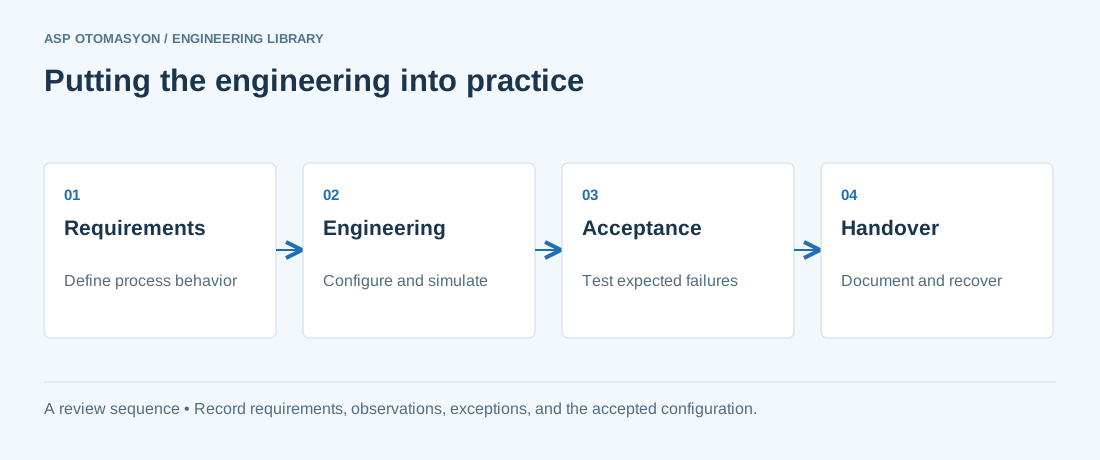
- Define the process states, timing requirements, and permitted behavior after a controller or communication failure.
- List controller, I/O, network, software, and license dependencies before choosing an architecture.
- Record acceptance results and prove that the delivered configuration can be restored from the handover package.
Follow an ASP project guide to connect the fundamentals with implementation and acceptance.
Primary references and further reading
Use the original specifications and product documentation for implementation details. The examples in this guide are illustrative engineering scenarios, not published project results.